
Saul
Friday, January 6, 2023
Part 2: Code implementation
Important
Although I try to keep this post updated, a number of changes were made to the code since the first publication which are not reflected in the description. I don’t think these modifications fundamentally change the purpose of description but it is recommended to check the source code hosted in GitHub for the latest changes
Summary
In this post the implementation of the extension of the degradome analysis is described. All the steps for sequencing-data processing, degradome analysis and report generation have been wrapped in two bash scripts 01-Degradome.sh and 02-Degradome.sh. The former’s main job is to map the sequencing data and run the PyDegradome script; which will compare pairs of samples (one with the factor thought to affect the production of degradation intermediates and another without it) and produce a table with genomic coordinates (peaks) where significant differences have been found. The job of the second script (02-Degradome.sh) is to process the PyDegradome data, first by associating the peaks with a particular gene and then by filtering and classifying these based on different ratios of read values within and between samples. An additional step was included where sequences around peaks are aligned to known miRNA sequences with the aim of identifying putative miRNA targets. This step do not make use of specialized software thus, the results should not be considered as high confidence miRNA targets.
Instructions are provided to set up the environments for the analysis, the variable definition file and the overall structure of files and folders to be able to replicate the analysis. Links to the code and custom packages are provided at the end of the post.
Overview of the scripts
All the steps for processing the sequencing files have been grouped into two bash scripts, 01-Degradome.sh and 02-Degradome.sh.
Briefly, the main step of the former is to map the sequencing files and use these as input to, run the PyDegradome script (Gaglia, Rycroft, and Glaunsinger 2015). The script compares pairs of samples, one with a factor thought to affect the production of RNA degradation intermediates and one without it. This comparison is carried under user-defined settings for the identification of significant differences most relevantly, a multiplicative factor (MF) for the production of degradation intermediates and a confidence level (CI) for the statistical tests. The pairs of samples to be compared and the settings to be tested are specified in the variable definition file (See Variable setup file). The output consist on a list of genomic coordinates (referred as peaks) where significant differences between samples were found.
The results of the above analysis are then processed by the second script, which in turn is a wrapper for a number of R scripts. Their function is to associate the identified peaks with a particular gene, filter and classify them into categories of candidate peaks. Two classifications steps are implemented based on ratios of read values from the peak region and those found outside it. Plots of reads found around the peak and all along the associated gene are produced as a way to provide visual evidence of the classification. In addition, sequences around the peak region are aligned to known miRNA species in order to identify putative targets. Finally all the information obtained is summarized in a html report which can be used for selection of candidates for further studies.
All the steps performed by each script are listed below and details of relevant ones are explained in latter sections.
01-Degradome
- 00 - Check for arguments
- 00 - Check for variables
- 00 - Check for files
- 00 - Check for indices Bowtie
- 01 - Fastq quality control 1
- 02 - Filter by length, trimm adapter and quality filter
- 03 - Fastq quality control 2
- 04 - Remove rRNA
- 05 - Fastq quality control 3
- 06 - Map to genome Tophat
- 07 - Convert bam to sam [Genome]
- 08 - PyDegradome
- 09 - Bam Quality check [Genome]
- 10 - Map filtered reads to transcriptome
- 11 - Extract uniquely mapped [Transcript]
- 12 - Convert sam to bam and create bam index [Transcript]
- 13 - Bam Transcript Quality check
- 14 - Count mapped reads to features [Genome]
- 15 - Count mapped reads to features [Transcript]
- 16 - Create 5 Wig track [Genome]
- 16 - Create 5’ Wig track [Transcript]
02-Degradome
- 00 - Check passed arguments
- 00 - Check variables
- 00 - Test if miRNA variables are available
- 00 - Initialization.R
- 01 - Annotation-shared_peak_classification.R
- 02 - Filtering_Classification_Pooling.R
- 03 - Drawing_Dplots.R
- 04 - GetPeakSeq.R
- 05 - Peak_miRNA_alignment.py
- 05 - Report-settings.R
01-Degradome.sh
The script must be called from input root folder with two arguments, the ‘Project Name’ and the ‘variable setup file’. The former should match the name of the output root folder and the latter the name of the variable definition file. No path declaration is needed. As an example, the code below was used to analyze the data from the work of Oliver et al. 2022, in this context the first author’s surname and year of publication was used for both parameters.
Upon execution, the script checks for at least one argument and echoes the string to be used as Project Name. If no argument is passed it exists. On the next step, variables and files found in predefined folders are checked; if not found, the script will attempt to create them by calling auxiliary scripts.
Out of all the steps listed for the first script, steps 01 to 05 are common to any mapping pipeline and can be freely modified (for example, omitting the removal of rRNA). Steps 06 and 07 are somehow mandatory in the sense that PyDegradome requires reads to possess a valid XS:A: tag (commonly assigned by the mapping program tophat) and for these to be in SAM format1.
PyDegradome
This represents the main step of the 01-Degradome script. It compares two samples (a test and a control) under user-defined settings for the statistical analysis including: a multiplicative factor2 for the production of mRNA fragments, a confidence interval used to set the threshold of significance and a window of nucleotides for reads to be combined when performing the comparisons. Additionally, the script requires an annotation file (*.gtf) and, optionally, an estimate for the total number of sites where reads can be found. The latter argument is used to estimate the number of sites with zero reads, \(S_0=S_t-S_1\) where \(S_t\) is the estimate of all potential sites that could have a read and \(S_1\) is the observed number of reads from the mapping data. Parameters for the probability distribution are estimated making sure that ’the probability of observing a zero read count (\(S_0\)) matches the data’ and it is advised that it may be necessary to change its value (default 32348300) when working with data from non-mammalian cells (PyDegradome README file Gaglia, Rycroft, and Glaunsinger 2015).
In the original script all the arguments must be passed in a particular order (positional) which may lead to some errors3 thus, a few modifications were made one to allow for named arguments and another related to how SAM’s CIGAR strings were parsed4. Because the analysis was run on a data sets from Arabidopsis, the code includes a step to obtain an estimate of the total number of sites; this by multiplying the length of the reference sequence (fasta file) times 0.01 (Code to run PyDegradome, lines 1-3). Interestingly, for the data sets tested in part 3 and part 4 of this post series, changing the estimate of total sites caused an error in the script (partly due to a slow convergence in the parameter estimation) while none was reported when the default value was kept. The only case where changing the value of the total sites (using the fasta_len value) proved to be useful was when the mapped data was restricted to a small chromosome such as the chloroplastic.
Lines 5-19 of the code shows the actual call to the PyDegradome script. First, it checks if one the output files (*.tab) exists5 before calling the script. The full code includes a call for the reverse comparison and it loops over all the samples and settings stated in the variable definition file.
Scaling of mapped reads
Reads mapped to both the genome and transcriptome are scaled before sample comparison. The scaling is performed with bamCoverage using as a scale factor the inverse of DESeq size factor. Reasons for choosing a scaling method over normalization are discussed on a post on deeptools forum.
Single chromosome analysis
If the analysis of a single chromosome is needed, a slightly different script was developed (01-degradome-ch.sh) where the chromosome to focus on is defined in the variable setup file. Using this script it is important to check that the chromosome names defined in the annotation file are the same as those used for the locus naming. In the case of Arabidopsis, chloroplastic and mitochondrial chromosomes are named Pt and Mt on the annotation file however, when referring to a locus these are replaced by C and M. Such situation is considered in the code during transcriptome mapping but it may have to be adapted for a different species.
fasta_len variable which is calculated as 0.01 of the length of the genome reference file.02-Degradome.sh
As with the first script, 02-degradome.sh requires two arguments, ‘Project Name’ and the ‘variable setup file’.
At first, the script will also check if variables have been defined. One difference however, is that the script will also look for a specific variable,miRNA. This points to the annotation file for precursors and mature forms of miRNAs of the species under study. If not defined the script will attempt to download a list of organisms from miRBbase match these against the species under study (defined in the variable definition file) and download the corresponding file.From this point on a series of R scripts are called to create necessary objects, annotate and classify peaks, plot these, etc. The main characteristics of these are described below.
Initialization
00-Initialization.R: It will import the variable definition file into R and save it as an .RData object to be used by the rest of scripts. While doing it a number of new variables will be defined; also, folders to store auxiliary files, intermediate output and the final report will be created.
Among the auxiliary files created it is worth mentioning:
txdb_object: A transcript database object build from the annotation file (*.GTF or *.GFF3) and used to match peak coordinates to a particular gene.Transcript_information.txt: A tab separated table created from plant ensembl Biomart used to distinguish the representative gene form. The latter is defined as “the model that codes for the longest CDS at each locus” (From TAIR10 )<specie>.sqlite: A Sqlite database used to transform genomic coordinates to transcript coordinates when running04-GetPeakSeq.Rscript
Whether these are adequate for the species under study should be checked before running the script.
Peak annotation and computing of ratios
01-Annotation-shared_peak_classification.R: The script is divided into 4 blocks:
- Annotation of peaks: Peaks are associated to a particular gene if their coordinates completely overlap with a gene feature
- Build a data frame with coordinates for regions with no peaks: Creates a table with coordinates outside the peak region. This is used to calculate the peak:background ratio
- Calculate peak to non-peak ratio: Obtains the highest read within peak and outside peaks to then calculate their ratio. At the same time a table with the read values is constructed to speed-up future calls (e.g. when comparing different program settings)
- Generate shared peak table: Peaks are classified as either shared or found in only one replicate. For the latter, the peak coordinates are used to measure reads on the opposite sample (‘missing peak’).
Obtaining the highest read in a particular region is a relatively straightforward operation. The main function (GetMaxRead) is based on one described in a post by Antonio Dominguez ( ).
The function isn’t particularly fast as it has to read the alignment file (in bigwig format) to obtain the read values. The processing time is greatly extended considering that it has to be done for each peak and ’non-peak’ region, for every transcript and repeated for all the comparisons and parameters tested (i.e. PyDegradome settings, MF and CI). In order to speed up the process, every time a region is evaluated, an entry is created in an auxiliary table (see below). On subsequent calls this file will be queried for matching indices (indx column which is the concatenation of locus and peak coordinates) in order to avoid reading the alignment file. This has been shown to greatly reducing the processing time but only when different PyDegradome settings are being compared.Classification of peaks as shared between replicates or unique to a particular one is a simple process that involves finding overlaps between coordinates. However, for those peaks found only on a single replicate an extra step is included in order to have a set of peak measures for both replicates (which will be latter used for the classification and filtering). A pseudo-peak is calculated for the replicate without measure using peak coordinates from the other replicate. This represents additional rounds of reading the alignment file and it also uses the auxiliary file to speed up the process.The main output of this script is a table with the combined data of the comparisons between test and control replicate 1 and 2, e.g. Comparison_SRR10759112-SRR10759114_and_SRR10759113-SRR10759115_0_95_4_2. The filename reflects, respectively, the two comparisons pooled, the values for the confidence interval, window size, and multiplicative factor.
Classification and pooling
01-Annotation-shared_peak_classification.R: It performs a filtering step followed by two classification steps:
- Filtering: A threshold for the read count defined as the mean of reads rounded up to the next integer value (\(\lceil \bar{x}_{max\: peak} \rceil\)) is used to filter out peaks with low counts.
- Classification/Filtering 1: Based on the peak:background ratio of test samples (\(Test_{max\: peak}:Test_{background}\)) arbitrary cutoff points are defined to classify the peaks into 4 categories (1-4) plus an extra category (0); the latter used for those peaks that could not be classified in the first four categories.
- Classification 2: A ratio is calculated between peaks of test samples and all the reads found on the corresponding controls. For test samples, the highest read within the peak region is obtained and the mean calculated (\(\bar{x}\: max\: read\: peak_{Test}\)). For control samples, the highest read along the transcript is obtained and the mean between replicates is calculated (\(\bar{x}\: max\: read\: transcript_{Control}\)). Finally a ratio between these two means is calculated and used to classify peaks in two categories (A and B) plus an extra one (C); the latter for those peaks that could not be classified into one of the first two categories.
Since the classification steps were some of the main additions to the degradome analysis, further details of these are given below
Filtering and classification 1
Peaks were classified into 4+1 categories based on the ratio of their highest point and the highest read found outside the peak region (peak:background).
- Category 1: The peak is identified in both replicates and represents the highest signal on the transcript.
- Category 2: The peak is identified in both replicates and it is at least 80% as high as the highest signal
- Category 3: The peak is identified in both replicates and it is at least 70% as high as the highest signal
- Category 4: The peak is identified in only one replicate and it is at least 80% as high as the highest signal on the transcript. Also, the signals found on the same coordinates for the other replicate are also at least 80% as high as the highest signal on the transcript.
- Category 0: Peak that can not be classified in any of the above categories.
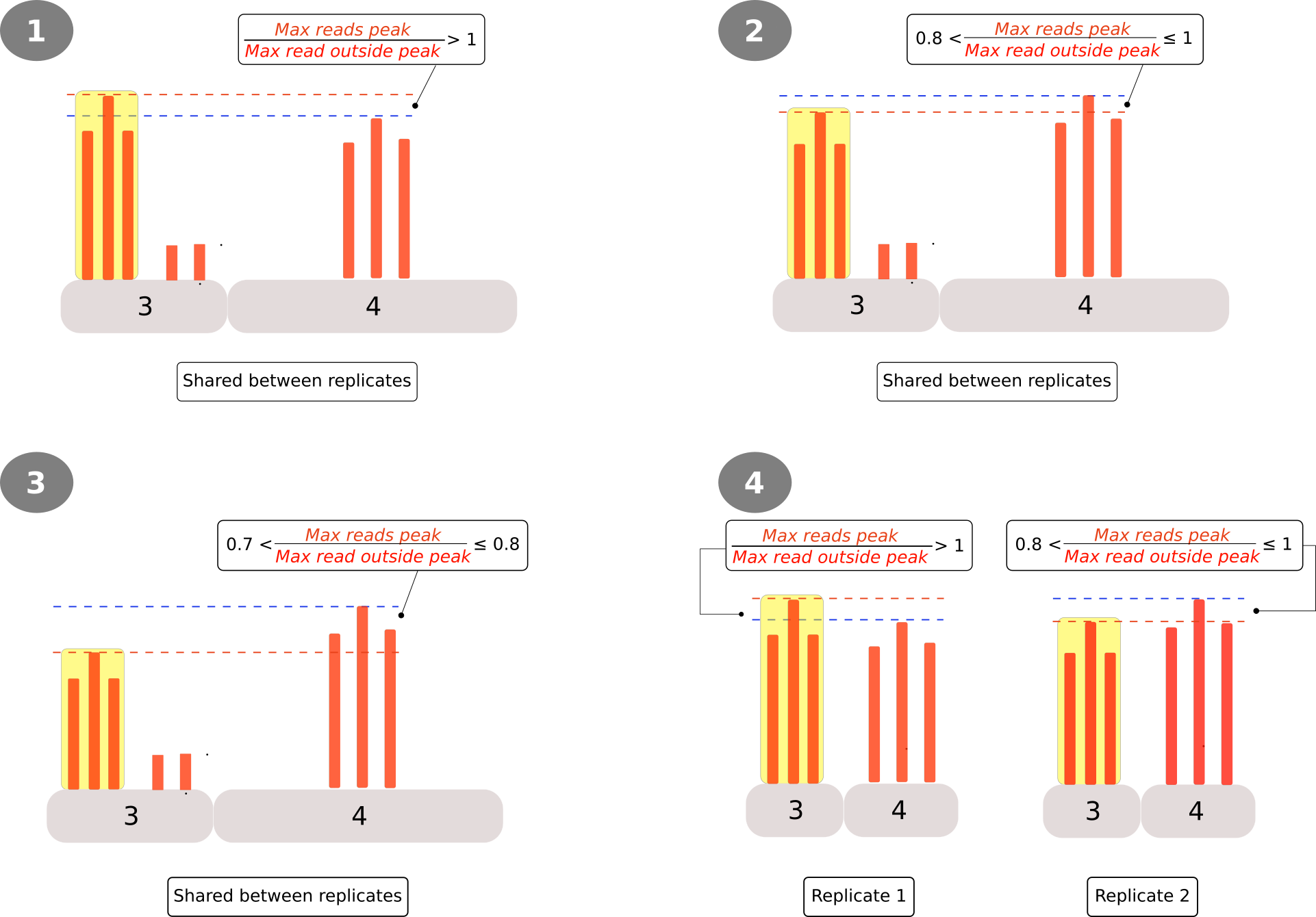
Figure 1: Criteria for the classification/filtering of peaks obtained from the PyDegradome analysis. A ratio between the peak’s reads (highlighted yellow) and those outside (background) was used to define 4 categories (Circled numbers). Categories 1 to 3 consider peaks found in both replicates while, category 4 analyzed peaks found only in one replicate. In the latter case, coordinates of the identified peak were applied on the other replicate as it were a significant ‘peak’
Finally peaks that could not be classified in one of the four categories were labeled as category 0.
Classification 2
Classification 1 does not consider the scenario where a read found in the control sample (in a region other than the peak) could be higher than that found in the peak region of the test sample. To account for such cases a second classification was included comparing the peaks found in test samples with all reads found in their corresponding controls. Reads were scaled using DESeq scale factor and the mean of the highest read, in the peak region (test samples) or all along the gene region (control samples) were divided. Based on the value of the ratio 3 categories were defined (Figure 2).
- Category A: Ratio is higher than one
- Category B: For those genes with two or more peaks the ratio between the mean value of the peak and the median value of the control is higher than one
- Category C: Peak that could not be classified in any of the above categories
It should be acknowledged that the definition of category B is much more arbitrary than any of the other categories (including those from classification 1). They were included in the code to accommodate a bona-fide control used in my study that had two peaks along the gene region. For one of them the reads in one of the peaks were considerable higher than any other along the gene in, both, the test and control sample thus, unless such category was devised the second bona-fide peak could not be separated. Due to this bias, for the analyzed data reported in these posts only peaks classified at the top (i.e. Category 1 and Category A) were considered.

Figure 2: Criteria for the second classification of peaks obtained from the PyDegradome analysis. A ratio between the highest read in the peak region of test samples(mean of scaled values, red bars) and the highest read along the transcript from control samples (light blue bar) were used to classify the peaks into 3 categories. Category A for peaks with a ratio greater than 1. Category B was designed for those transcripts with more than 1 peak, where the ratio was higher than the median value of control samples. Finally category C included all the candidates that could not be classified in the two categories above. No candidates were removed from further analysis.
The results of the classification are appended to the previous table and saved using the preffix Classification (e.g. Classification_SRR10759112-SRR10759114_and_SRR10759113-SRR10759115_0_95_4_2). However, the main output and the one used for subsequent steps is a file combining all the comparisons, e.g. Pooled_0_95_4_2.
Drawing of D-plots
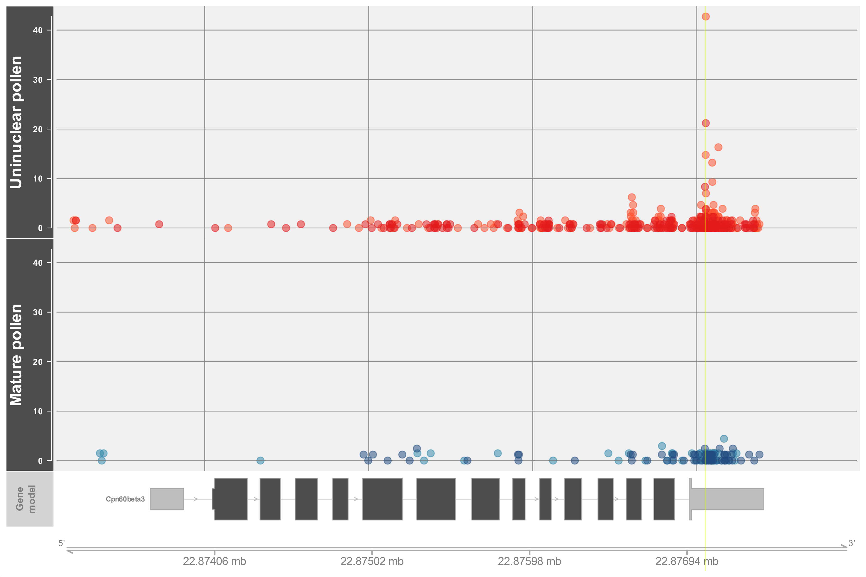
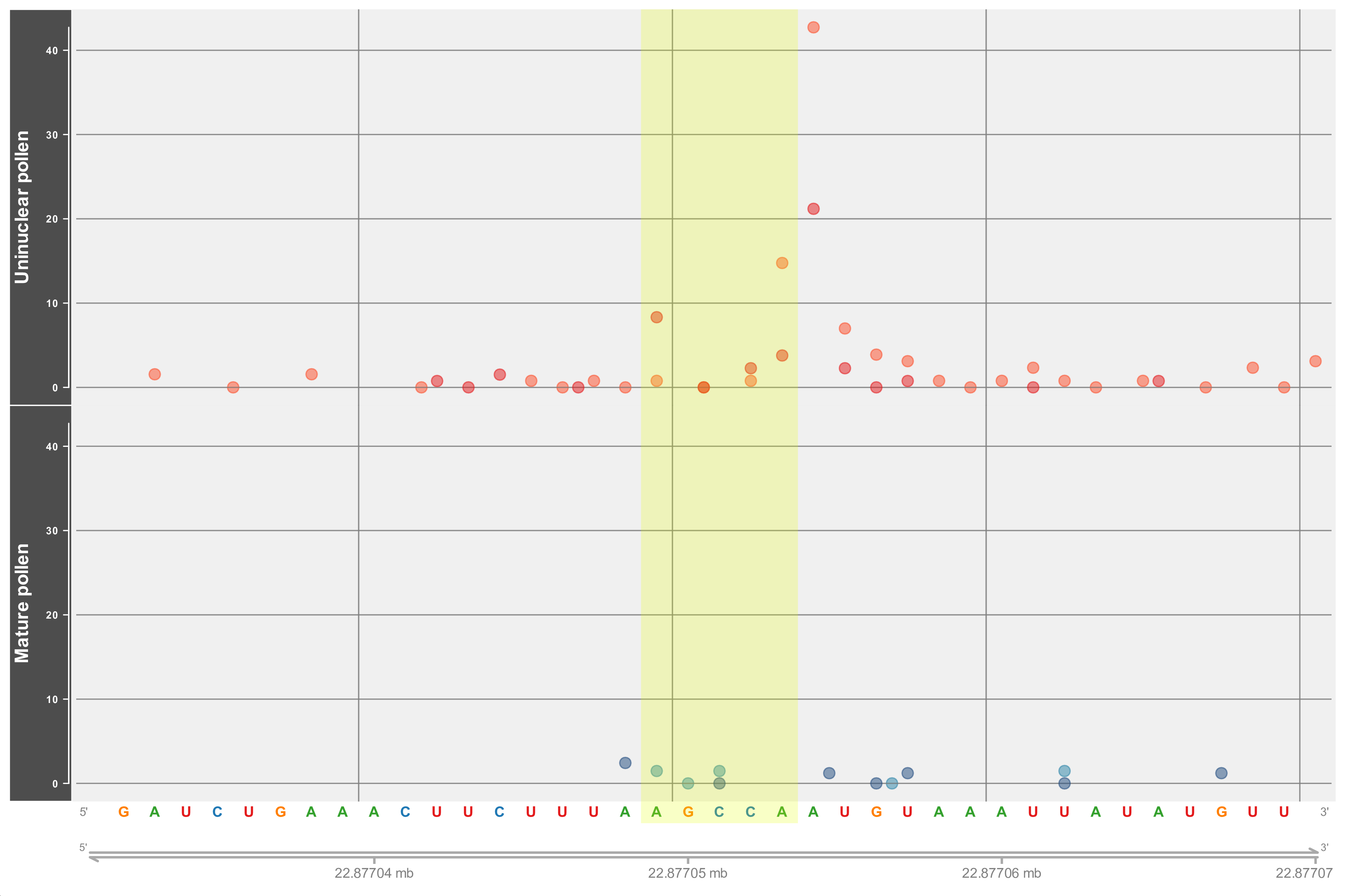
03-Drawing_Dplots.R: It draws two types of plots, one with all the reads mapped along the gene (Gene decay plot) and another focused on the reads found within a 40nt window around the peak (Peak decay plot). The former allows the comparison between the peak and the rest of the reads present along the gene region and can be used to validate the classification. For the example, the highlighted region shown in the gene decay plot below is misleading since it comes from a peak classified into category 0-C that is, from a peak that could not be classified in either of the two categories (or in other words one that could be discarded) however, the highlighted region (downstream of coordinates 2287694) seems to mark the highest read along the gene. Inspection of the peak decay plot supports the classification by showing that the peak region is actually next to the highest reads. Moreover, since the plot around the peak region shows the sequence it could also be useful in confirming the alignment with a particular miRNA.
Gviz with many of its parameters wrapped in a custom function (drawDplot). Note that the code is long and the function call takes many parameters. This was necessary in order to allow the function to draw the two types of plots. Regarding the function call, the parameters that need to be changed for the function to draw a ‘peak plot’ are commented and highlighted.Note that Gviz has a lot of options for changing the aesthetics of the plot but only a few can be modified from the function call. Worth mentioning are the ticksn and i_factor parameters which control respectively, the number of genome coordinates shown (i.e. tick marks) and the offset area to plot. Regarding the former early attempts rely on Gviz internal calculation of the number and position of the tick marks which led (in some cases) to overlapping coordinates. To solve this, two functions were written (GetPlotMarks and GetPlotCoors) however, it should be noted that they limit the number of marks to the range of 4-6. As for the latter argument (i_factor) it represents a proportion of the transcript width to be added at both sides. Lower values than the default may cover the gene name.Alignment of miRNA to peak sequences
These steps were not included on the original work but were added after analyzing the data in Oliver et al. 2022; and Zhang et al. 2021 both focused on miRNA targets. Using only those peaks classified in the highest categories (i.e. 1-A), sequences around them were obtained6 and aligned to known miRNAs. The alignment was performed using two different approaches, the simplest one performed a global pairwise-alignment (Implemented in biopython V.1.75 Cock et al. 2009) using a 22nt region centered around the peak whereas, the second one used a program that predicts the strength of the interaction between a miRNA and a putative target (Mirmap Vejnar and Zdobnov 2012); in this case a longer sequence around peaks (40nt) was compared to known miRNAs. For both approaches, an alignment file for the corresponding species was downloaded from TarDB (Liu et al. 2021). and used as input for the alignment programs. Alignment scores were obtained and their lowest values used as threshold for the selection of candidates.
Global alignment
05-Peak_miRNA_alignment.py: The script defines a function to check the length of the miRNA and trim the peak sequences (\\(Len\_{miRNA}+2=Len\_{Trimmed peak seq}\)) before conducting a global alignment using biopython’s Align module. The alignment uses a nuc44 matrix, a gap open penalty of -10 and an extension penalty of -2. Alignments with a score equal or higher than 33 are selected. The threshold was chosen after performing the same alignment7 using all the sequences from the miRNA alignment and observing the summary of all the alignment scores, as shown below.
| Variable | Value |
|---|---|
| count | 3510.000000 |
| mean | 65.556125 |
| std | 12.009904 |
| min | 33.000000 |
| 25% | 57.000000 |
| 50% | 63.000000 |
| 75% | 72.000000 |
| max | 105.000000 |
mirmap. Length of the seed sequence was set to 11-12nt; note that out of the 3510 pairs of sequences only 557 used by the program.| Variable | Value |
|---|---|
| count | 557.000000 |
| mean | -22.722442 |
| std | 4.154223 |
| min | -36.299999 |
| 25% | -25.500000 |
| 50% | -22.100000 |
| 75% | -19.799999 |
| max | -13.800000 |
At the end of this step three types of files are produced, a serialized object (Alignment_indices_MF-<MF>_iConf-<CI>.obj), a text file (miRNA_targets_MF-<MF>_iConf-<CI>.txt) and a number of images showing the alignment between sequences (Aln-global-<ATxGxxxxx>-x-ath-miRxxx-<CI>-<MF>.png). The former contains a nested list with the indices of miRNA and peak sequences and the score of the alignment which can be used to for further inspection or for troubleshooting. The second file contains a list of transcripts whose associated peak sequence aligned with a particular miRNA (see miRNA candidate targets). The sample comparison where the peak was identified and the alignment score is also reported. Finally, for the selected alignments an image is produced with the base-pairing and the alignment score.
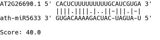
Figure 5: Example of a peak sequence selected after a global alignment against known miRNAs. Alignment score is reported at the bottom.
miRmap alignment
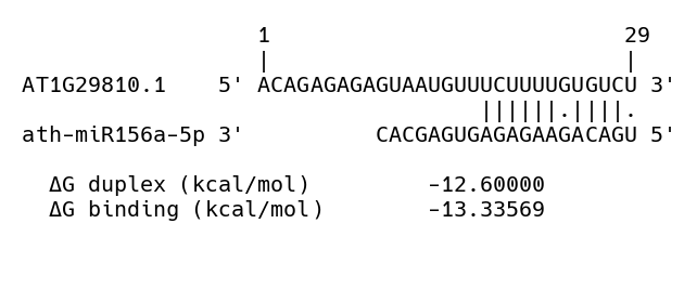
05-Peak_miRNA_mirmap.py: Aligns a sequence of 40nt centered around the peak region against known miRNA sequences using the python program mirmap (Vejnar and Zdobnov 2012). The program searches for potential miRNA targets using a seed region (a sub-sequence starting at the 5’ end of the miRNA) that is aligned against a target sequence. For the best match a number of predictors (thermodynamic, evolutionary, probabilistic or sequence-based) can be computed however, only the thermodynamic are used since they are considered to be independent of the species on which the program was developed (i.e. Human and mouse). Two values are reported, \(\Delta duplex\) and \(\Delta binding\). From the program description (Vejnar and Zdobnov 2012), the former represents the “minimum folding energy (MFE) of the miRNA-mRNA duplex, calculated using Vienna RNA secondary Structure library” whereas, the latter, represents the folding energy of a sub-optimal structure. The length of the seed sequence used for the identification of targets was set to 11-12 (higher than the default of 6-7) allowing either a G:U wobble or a mismatch in either position. As a reference pairs obtained from the alignment of miRNA with their verified or predicted targets were used as input. Note in the summary table above that out of all the 3510 miRNA-mRNA pairs used for the global alignment, only 557 could be aligned using mirmap. Because of this, the values for the \(\Delta duplex\) were used only as a reference rather than a threshold.
As with the global alignment, the results of this step are recorded in three different files, a serialized object (mirmap_indices_MF-_iConf-.obj), a text file (mirmap_miRNA_targets_MF-_iConf-.txt) and a number of images showing the alignment between sequences (Aln-mirmap--x-ath-miRxxx--.png). The only difference is that the alignment file reports the positions in the peak sequence (within the 40nt window) where the alignment was detected and the thermodynamic parameters of the duplex instead of the alignment score.
Report generation
An html report summarizing all the classification steps, listing the candidate peaks and all the putative miRNAs that are likely to target the peak regions is produced by 3 different files:
- 05-Report_main.R
- 05-Report.Rmd
- 05-Report_code.R
The former loads all the necessary packages, and loops over the settings used for the PyDegradome analysis while calling the second script. This is an Rmarkdown file whose main function is to evaluate different code chunks present in the last file and produce the report.
The last script will import the following files:
- The summary of counts (
/output_02/03-Report/Summary/Peak_counts_BeforeAfter_Filtering) - The table of peaks with all the information pooled (e.g.
/output_02/02-PyDegradome_pooled/Pooled_0_95_4_2) - Files all the miRNA targets identified (e.g.
miRNA_targets_MF-2_iConf-0_95.txtandmirmap_miRNA_targets_MF-2_iConf-0_95.txt, both located in /Supporting_data/miRNA_seq/output)
Processing of these files will result in three tables in the html report with the ‘List of candidate peaks per comparison’ containing the main information. All the data from the annotation and classification steps is divided into 3 tabs (General classification, Classification (Metrics) and Coordinates) to avoid showing too much information at once. Candidate peaks are grouped by the sample comparison (e.g. Mature pollen vs Unicellular pollen) sorted by the two classification categories (combined in the first column) and the ratio Peak(T):Max(C) (See Peak annotation and computing of ratios). Links to peak and gene decay plots are included.
Finally, the list of putative miRNA targets will list all the transcripts identified from either of the miRNA alignment approaches. The list is sorted by the global alignment score followed by the value of \(Δ\)G open from mirmap. Links to the sequence alignment and for the peak-decay-plot are provided in order to compare the alignment with the mapped reads. Missing alignments are indicated by the icon .File and Folder structure
The whole analysis pipeline uses and generates many files and folders. In an attempt to keep these in order, a specific file and folder structure was defined for both the input and the output. Most of these are defined in the variable setup file (see below) while others are defined in the 00-Download-genetic-data.sh and 00-Initialization.R scripts. Those defined in the scripts are hard coded and it is recommended to keep them as they are.
Variable setup file
In this file most of the variables and files used by the scripts are defined. It must be located in the Env_variables folder.
The template below has been organized in order of importance with variables that must be defined by the user at the top and others that can be kept unmodified at the bottom.
Input and output directories are defined first. Both can be set to any destination however, note that the output folder has been set to have the name, Degradome-${ibase} where ${ibase} corresponds the project name which is passed as an argument when executing the script.
*_samples_name variable will be used for drawing plots and during report generation and should have the same base name with only the replicate number indicated between brackets6. Note that the variable pydeg_comp_list is an array with test-control pairs.The Species related variables (lines 30-35) are used when downloading annotation and sequencing files; the variable ver (note the leading dot in the assigned value) represents the current version of the file at the time of writing the post.
As for the anaconda environments make sure all the environments exits (see Anaconda environment setup)
Regarding the annotation files make sure that the final name matches those where the files will be downloaded from or (if already downloaded) copy them to the correct folder,Annotation/ and set up the variable accordingly. For the former case, the values specified in the template above match the file names in ensembl (for example ).Finally a note that some of the values of variable names that do not require modification are hard-coded (e.g. output_01). Before modifying them check the overall folder structure, particularly of the input files/folders.
Input files/folders
The whole input folder/file structure for the analysis is shown in the tree below. If cloned from the repository, it should already be set up except for the annotation files (red branch) which are downloaded/created while running the scripts. The root folder (<input-dir>) could be given any name and placed anywhere just note that the size of the whole tree could be around 2GB due to the sequencing files, which will populate the Genetic_data sub tree. Colored in green is the path to the variable setup file; in this case named using the last name of the author and the year of the work. Finally colored purple are all the auxiliary scripts, they have been grouped by the language and by their source with the third_party folder containing the modified PyDegradome script and the mirmap files.
Output files/folders
The tree below illustrates the structure for the output. Unlike the input structure the root of the tree can not be named arbitrarily; it must conform to the string Degradome-<project-name> where <project name> is the same as the first parameter passed to the main scripts (e.g. Oliver-2022). The rest of the tree is setup by the scripts with the only exception being the subfolder output_01/01-fastq which must be created in advance and should contain the raw sequencing files.
As described above the output_01 sub tree will contain the files produced during the mapping and PyDegradome analysis; the latter representing the main step of this part. In the sample output tree the files for a single comparison are shown in the 05-PyDegradome folder; those with .txt and .tab extensions are auxiliary files whereas, that with no extension (t_SRR10759112_c_SRR10759114_0.95_4_2) contains main output. The filename includes the name of the sequencing files used as test and control, respectively, the confidence interval, the width of the window of nucleotides, and the value of the multiplicative factor.
As for the output_02 sub tree it contains the results from further processing the PyDegradome results and are considered the main files produced by the whole analysis. They include the html report, Report Degradome Analysis Oliver-2022_MF-4_Conf-0_95_Oliver-2022.html and many intermediary files that could be used for troubleshooting or improving the report.
Briefly, the files contained in the 02-PyDegradome_pooled are all tab-separated files with the following characteristics.
- Comparison: A table with the results of two sample-comparisons pooled
- Classification: The table above plus the information about the classification of their peaks
- Pooled: A table combining all the comparisons tested
Concerning the Summary folder (green branch at the bottom), it contains different files summarizing the classification and filtering of peaks:
Annotated_peak_number: A table with all the peaks that were associated with a genePeak_counts_BeforeAfter_Filtering: A table with the number of peaks remaining after each classification step and on the last column focusing on the top classification (categories 1 and A)Peak_counts_classification-1: A table with the peak count in each of the categories defined for classification 1Peak_counts_classification-2: A table with the peak count in each of the categories defined for classification 2
Finally, regarding the files and folders contained in the Supporting_data sub tree (red branch) they include:
Degradome_reads: Contains tables with max-read-counts for peak and non-peak regions which are used to speedup the calculation of ratios.miRNA_seq- input: Contains the miRNA sequences used for the alignment
- output: Contains the files with miRNA sequences and the python objects with the alignment indices and scores
Peak_sequences: Contains fasta files with sequences around peakspyDegradome_maxPeak_Scaled: Contains tables with max-peak-counts (scaled values)pyDegradome_maxTx_Scaled: Contains tables with max non-peak reads (scaled values)pyDegradome_NonPeaks_coordinates: Contains tables with non-peak coordinatesR: A number of R objects such as variables and package specific objects (see the Initialization section)
Anaconda environment setup
Tools used for the analysis of the data were installed in three different anaconda environments (miniconda installation)
- pydeg_map: Used for most of the steps of script 01-Degradome.sh
- pydeg_run: Used only to run the PyDegradome script using
- pydeg_R: Used only to run R scripts
The code used to set up these environments is described below
Main environments
The following commands will create all the anaconda environments mentioned above and install the required packages within them. Linux dependencies needed to install and setup R are indicated at the beginning.
R package installation
The following commands should be run on the environment pydeg_R. They will install bioconductor and all the packages required for the analysis of the data. Note that the version of bioconductor should be compatible with that of R (See bioconductor installation instructions).
Custom package installation
A number of commands used to process the data were wrapped in an R packaged named R_PostPydeg available at GitHub. The commands to install it are described below. Note that this must be done inside the pydeg_R environment.
Final thoughts
Scripts 01-Degradome.sh and 02-Degradome.sh are an attempt to expand the analysis of the original PyDegradome script (Gaglia, Rycroft, and Glaunsinger 2015) though the addition of a series of classification and filtering steps that result in a list of transcripts with degradome signals (peaks) considered as likely candidates. Information is summarized in a html report aimed to facilitate the inspection of these candidates. I applied it first to analyze a putative mRNA endonuclease and, in these post series, I tried to test it on data from miRNA studies, (Oliver et al. 2022; Zhang et al. 2021). In this context an extra step was included to align sequences around the peak region with known miRNA species.
The overall code could be considered nothing more than an exercise since in plants there is not a report on a bona fide RNA endonuclease; and there are plenty of specialized programs for the analysis of miRNA targets (See the introduction section in Thody et al. 2018). However, while writing and testing the code it was noticed that in some of the studies on degradation intermediates the idea of finding targets in 2 or more replicates is often overlooked. Less often is the comparison between samples where are clear difference is presented. The latter concept is central to the code presented, whereas the former, is emphasized in the original work by Gaglia, Rycroft, and Glaunsinger 2015. In this context, the above analysis could be regarded as an additional source for candidate selection.
Care has been put on trying to make it as error-free as possible and to make it as general as possible; so it could be adapted to other species besides Arabidopsis without significant modification yet, no warranty is provided.
The scripts and the custom R-package are hosted on a public github repository (see below)
References
Code availability
Web resources
- Post cover image:
- Artist: luis gomes
- License:
Alternatively tophat could be set not to convert the mapping files but BAM files are still needed in downstream steps. ↩︎
It can be considered as analogous to a fold-change in convetional RNAseq analysis ↩︎
Before changing to named parameters I was getting an error when trying to set the optional parameter -t (estimate total number of sites) ↩︎
PyDegradome uses SAM’s CIGAR strings to determine the starting position of a mapped read. In the original script, those reads with a FLAG value of 16 (SEQ being reverse complemented) and with a XS:A: field with a negative value (-) were considered only if its CIGAR string contained only an M (matched or mismatch) or an N (skipped from reference) operation. The modified script extends5 this to allow CIGAR strings with the additional operands, \(=\), X, P and S. The idea behind the modification was to use other mapping software such as STAR however, many reads mapped by this program lack the XS:A: field which is needed by PyDegradome. Since there is no difference in how CIGAR strings with only M and N operands are processed by this modification, it was kept. ↩︎
: The modifications were based on edgardomortiz’s sam2consensus.py script more specifically, the
parsecigarfunction. ↩︎ ↩︎Peak sequences (40nt) centered around the highest peak point are produced while running 02-Degradome.sh, specifically when calling the auxiliary script 05-Get_miRNA_seqs.sh. They are located in the /Supporting_data/Peak_sequences folder. ↩︎ ↩︎
An auxiliary script specifically for this step is included in
<input_dir>/>Scripts/sh_py/00-mirTarget_alignment. It assumes that both sequence filesath_mir.faandath_tar.fa(see code Genetic_data/Fasta) are located in theGenetic_data/Fastafolder. ↩︎